This article follows the earlier tutorial on stochastic processes. It talks about a couple of related things, and tries to provide an intuitive understanding of some of the following concepts:
- Continuous returns and discrete returns models of stock prices,
- An understanding of how volatility affects the net realized returns obtained by an investor, and how the ‘average’ of discrete returns over a period of time can be misleading,
- How the true returns obtained by an investor are driven lower by the volatility of the discrete returns,
- The difference between log returns and discrete returns, and how the two are related, and
- Why is the formula for expected stock prices in the future
 and not e^(mu+sigma^2 /2)
A brief recap to the earlier tutorial on Stochastic Processes would be in order. Recall that a ‘Markov process’ is a stochastic process where only the current price drives the future price. Historical prices, or trends are not important. For Markov processes, the variances of changes in the variable (note: changes in the variable, not the variable itself. In other words, returns, not price) are additive.
A ‘Wiener process’ is a type of Markov process with mean=0 and standard deviation = variance = 1. For us, a Weiner process is nothing but a standardized normal distribution.
Take a stock. Stock prices are driven by hourly, daily, weekly (or periodic) returns that add to the initial price. Stock prices are lognormally distributed, and stock returns are normally distributed. The mean of the stock price, and the mean of the returns are obviously completely different things. However, the volatility of the returns is equal to the volatility of the price. (This makes logical sense if you think about the formula for standard deviation. Once you take the constant out, you are only left with the delta, or the changes, ie the returns.)
The way stock prices work is as follows. If ΔS is the change in price, μ the returns for one time period, and σ the volatility for the same time period, then the expected change in price for the time period dt is defined as follows:

Where dt is the time (a very short period of time), and dz is the Weiner process. What we mean by ‘dz is the Weiner process’ is that dz is replaced in the above equation by a random number drawn from a standard normal distribution. This number can be randomly drawn, and in Excel we can draw a random number from a normal distribution using the formula = NORMSINV(RAND()).
If we were to use discrete rates, the formula would be just slightly different.

where ϵ is a random drawing from the normal distribution.
The difference between the two: The thing to note is that Δt is a short period of time, while dt refers to time in a continuous, instantaneous sense. So long as Δt is short, there is practically no difference between the discrete and continuous time versions of the stock price model.
How do you interpret standard deviation for a stock? Consider a stock with a starting price of $100 that returns 10% a year, with an annual volatility of 25%. This means the stock’s returns over one month can be modeled as:

where ϵ is a random draw from a normal distribution. As mentioned before, ϵ can be simulated in Excel using the formula =NORMSINV(RAND()).
Note that Δ S is the change in price, in dollars, and not as a percentage. Because stock returns really only make sense as a percentage of initial price, we can divide both sides of this equation by S to get the percentage change in price.
Therefore
Applying this to our hypothetical stock with an annual return of 10% and volatility of 25%,
,![]()
Since we know ΔS, and we know ![]() , we can easily figure out
, we can easily figure out ![]() , which is the price at the end of period 1 as S + Δ S.
, which is the price at the end of period 1 as S + Δ S.
Mean and volatility of stock prices
If returns are normally distributed, stock prices are lognormally distributed. This follows from the definition of the normal and lognormal distribution,
We always talk about the mean and standard deviation of the returns. But what about the mean and standard deviation of the stock price itself? Well, the volatility of the stock price is the same as the volatility of the continuous returns. So that is easy. How about the mean of the distribution of the stock price?
But before we go there, a small digression would be interesting.
The difference between discrete and continuous returns, and how volatility hurts
If and are the prices at times 1 and 0 respectively, then discrete returns are calculated as ![]() , whereas continuous returns are calculated as
, whereas continuous returns are calculated as ![]() . Are continuous and discrete returns the same? For very short intervals of time, they are almost the same. In other words,
. Are continuous and discrete returns the same? For very short intervals of time, they are almost the same. In other words, ![]() . But over time, they are not the same. If you have a large number of time periods, then the mean of discrete returns can be misleadingly higher than continuous returns.
. But over time, they are not the same. If you have a large number of time periods, then the mean of discrete returns can be misleadingly higher than continuous returns.
For example, consider the following two income streams from a fund manager.
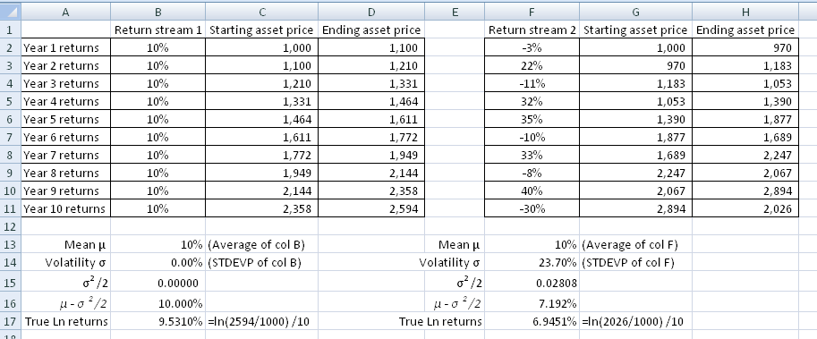
In both cases, the ‘average’ discrete returns are identical at 10% a year. But their volatilities differ a great deal, which means that the ultimate outcome for the investor is different. An initial investment of $1000 grows to $2594 in the first stream, whereas it only grows to $2026 in the second case. What is happening? This is an illustration of the fact that the average of [ ![]() ] is much greater the average of [
] is much greater the average of [![]() ].
].
In the end, the investor only receives the real log returns, or the continuous returns. So how do we connect discrete returns to continuous returns? When we are told average returns for an asset are μ, what is μ? Is it the discrete return, or the continuous return? μ is almost always the discrete return, ie the ![]() variety, unless specified otherwise. For most questions, there may be no real way to know. In fact it does not even matter much because for short time periods, say daily returns, they are almost identical (ie,
variety, unless specified otherwise. For most questions, there may be no real way to know. In fact it does not even matter much because for short time periods, say daily returns, they are almost identical (ie, ![]() ). (Try it in Excel, taking the daily return equivalent of 5% annual returns.)
). (Try it in Excel, taking the daily return equivalent of 5% annual returns.)
The thing to note in the above numerical example with the two return streams is the fact that greater volatility has brought down the effective return quite significantly. Even though the “average” is still 10% in the second case, the net realized return is significantly lower. Can we quantify how much lower does volatility bring the return down to? Yes, it seems we can. The log returns (ie the continuously compounded returns) for a given μ and volatility σ are ![]() .
.
Ie, in other words, the higher the value of σ, lower are the continuous returns for a given μ.
If μ represents discrete returns that are normally distributed with a volatility of σ, then log returns are normally distributed with a mean of ![]() and standard deviation of σ. How exactly this value of is derived is using a mathematical result by the name of “Ito’s Lemma”. The mathematical proof of Ito’s Lemma and its application to the modeling of stock prices is beyond the scope of the PRM (and also the mathematical abilities of this author).
and standard deviation of σ. How exactly this value of is derived is using a mathematical result by the name of “Ito’s Lemma”. The mathematical proof of Ito’s Lemma and its application to the modeling of stock prices is beyond the scope of the PRM (and also the mathematical abilities of this author).
Does this result hold out in practice? If for our given two income streams, are the log returns really equal to ![]() ? Well, Ito’s Lemma says it should be, but we can easily test it out in Excel. Consider the second income stream in the example above. If we calculate
? Well, Ito’s Lemma says it should be, but we can easily test it out in Excel. Consider the second income stream in the example above. If we calculate ![]() , we get close to the value of the log returns. But you will notice it is not identical, in fact it is significantly different. Why? Because our time period is quite large (1 year) and we have only 10 years. As Δt→ 0, we find that this relationship holds. As an example, break down the yearly returns into monthly returns over 5 years and then perform this calculation based upon monthly returns, and you will get pretty close. If you create a large series of returns, say using 100,000 rows, calculate the asset prices and compare the log returns to , using μ from the ‘average’ discrete returns, you will get the same results to many places of decimal. Ito’s Lemma gives us the formula for the mean of log returns for
, we get close to the value of the log returns. But you will notice it is not identical, in fact it is significantly different. Why? Because our time period is quite large (1 year) and we have only 10 years. As Δt→ 0, we find that this relationship holds. As an example, break down the yearly returns into monthly returns over 5 years and then perform this calculation based upon monthly returns, and you will get pretty close. If you create a large series of returns, say using 100,000 rows, calculate the asset prices and compare the log returns to , using μ from the ‘average’ discrete returns, you will get the same results to many places of decimal. Ito’s Lemma gives us the formula for the mean of log returns for ![]() as equal to
as equal to ![]() .
.
Future value of stock prices
If x is normally distributed with a mean of α and a standard deviation of β, then e^x is lognormally distributed with a mean of ![]() and variance of β. That is a property of lognormal distributions. (I used α and β instead of μ and σ to distinguish this generalization from the returns and prices example to follow.)
and variance of β. That is a property of lognormal distributions. (I used α and β instead of μ and σ to distinguish this generalization from the returns and prices example to follow.)
In our stock prices case, returns are normally distributed with a mean of μ and standard deviation of σ. Therefore log returns are normally distributed with a mean of ![]() and standard deviation of σ. Thus a lognormal distribution based upon this normally distributed returns variable will have a mean of
and standard deviation of σ. Thus a lognormal distribution based upon this normally distributed returns variable will have a mean of ![]() and standard deviation of σ.
and standard deviation of σ.
In other words, expected future price of stock will be ![]()
That’s it folks for now. Thank you for reading!