This is a quick write up on eigenvectors, eigenvalues, orthogonality and the like. These topics have not been very well covered in the handbook, but are important from an examination point of view.
Eigenvectors, eigenvalues and orthogonality
Before we go on to matrices, consider what a vector is. A vector is a matrix with a single column. The easiest way to think about a vector is to consider it a data point. For example, if ![]() is a vector, consider it a point on a 2 dimensional Cartesian plane. If there are three elements, consider it a point on a 3-dimensional Cartesian system, with each of the points representing the x, y and z coordinates. This data point, when joined to the origin, is the vector. It has a length (given by
is a vector, consider it a point on a 2 dimensional Cartesian plane. If there are three elements, consider it a point on a 3-dimensional Cartesian system, with each of the points representing the x, y and z coordinates. This data point, when joined to the origin, is the vector. It has a length (given by ![]() , for a 3 element column vector); and a direction, which you could consider to be determined by its angle to the x-axis (or any other reference line).
, for a 3 element column vector); and a direction, which you could consider to be determined by its angle to the x-axis (or any other reference line).
Just to keep things simple, I will take an example from a two dimensional plane. These are easier to visualize in the head and draw on a graph. For vectors with higher dimensions, the same analogy applies.
Consider the points (2,1) and (4,2) on a Cartesian plane. These are plotted below. The vectors that these represent are also plotted – the vector ![]() is the thinner black line, and the vector for
is the thinner black line, and the vector for ![]() is the thick green line.
is the thick green line.
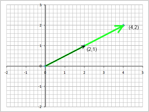
One of the things to note about the two vectors above is that the longer vector ![]() appears to be a mere extension of the other
appears to be a mere extension of the other ![]() vector. As if someone had just stretched the first line out by changing its length, but not its direction. In fact in the same way we could also say that the smaller line is merely the contraction of the larger one, ie, the two are some sort of ‘multiples’ of each other (the larger one being the double of the smaller one, and the smaller one being half of the longer one). We take one of the two lines, multiply it by something, and get the other line. That something is a 2 x 2 matrix. In other words, there is a matrix out there that when multiplied by
vector. As if someone had just stretched the first line out by changing its length, but not its direction. In fact in the same way we could also say that the smaller line is merely the contraction of the larger one, ie, the two are some sort of ‘multiples’ of each other (the larger one being the double of the smaller one, and the smaller one being half of the longer one). We take one of the two lines, multiply it by something, and get the other line. That something is a 2 x 2 matrix. In other words, there is a matrix out there that when multiplied by ![]() gives us
gives us ![]() . Let us call that matrix A.
. Let us call that matrix A.
For this matrix A, ![]() is an eigenvector. The extent of the stretching of the line (or contracting) is the eigenvalue.
is an eigenvector. The extent of the stretching of the line (or contracting) is the eigenvalue.
Now without calculations (though for a 2×2 matrix these are simple indeed), this A matrix is ![]() .
.
To explain this more easily, consider the following:
That is really what eigenvalues and eigenvectors are about. In other words, Aw = λw, where w is the eigenvector, A is a square matrix, w is a vector and λ is a constant.
One issue you will immediately note with eigenvectors is that any scaled version of an eigenvector is also an eigenvector, ie ![]() are all eigenvectors for our matrix A =
are all eigenvectors for our matrix A = ![]() . So it is often common to ‘normalize’ or ‘standardize’ the eigenvectors by using a vector of unit length. One can get a vector of unit length by dividing each element of the vector by the square root of the length of the vector. In our example, we can get the eigenvector of unit length by dividing each element of
. So it is often common to ‘normalize’ or ‘standardize’ the eigenvectors by using a vector of unit length. One can get a vector of unit length by dividing each element of the vector by the square root of the length of the vector. In our example, we can get the eigenvector of unit length by dividing each element of ![]() by
by ![]() . So our eigenvector with unit length would be
. So our eigenvector with unit length would be ![]() .
.
Calculating the angle between vectors: What is a ‘dot product’?
The dot product of two matrices is the sum of the product of corresponding elements – for example, if ![]() and
and ![]() are two vectors X and Y, their dot product is ac + bd.
are two vectors X and Y, their dot product is ac + bd.
Or, X.Y = ac + bd
Now dot product has this interesting property that if X and Y are two vectors with identical dimensions, and |X| and |Y| are their lengths (equal to the square root of the sum of the squares of their elements), then![]() .
.
Or in English,
![]()
Now if the vectors are of unit length, ie if they have been standardized, then the dot product of the vectors is equal to cos θ, and we can reverse calculate θ from the dot product.
Example: Orthogonality
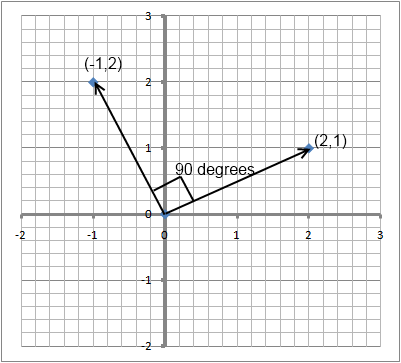
Consider the following vectors:
![]() . Their dot product is 2*-1 + 1*2 = 0. If theta be the angle between these two vectors, then this means cos(θ)=0. Cos θ is zero when θ is 90 degrees. Therefore these are perpendicular. And you can see this in the graph below.
. Their dot product is 2*-1 + 1*2 = 0. If theta be the angle between these two vectors, then this means cos(θ)=0. Cos θ is zero when θ is 90 degrees. Therefore these are perpendicular. And you can see this in the graph below.
For the exam, note the following common values of cosθ :
- Cos(90 degrees) = 0 which means that if the dot product is zero, the vectors are perpendicular or orthogonal. Note that the vectors need not be of unit length.
- Cos(0 degrees) = 1, which means that if the dot product of two unit vectors is 1, the vectors are overlapping, or in the same direction
- Cos(60 degrees) = 0.5, which means if the dot product of two unit vectors is 0.5, the vectors have an angle of 60 degrees between them.
If nothing else, remember that for orthogonal (or perpendicular) vectors, the dot product is zero, and the dot product is nothing but the sum of the element-by-element products.
Why is all of this important for risk management?
Very briefly, here are the practical applications of the above theory:
- Correlation and covariance matrices that are used for market risk calculations need to be positive definite (otherwise we could get an absurd result in the form of negative variance). IN order to determine if a matrix is positive definite, you need to know what its eigenvalues are, and if they are all positive or not. This is why eigenvalues are important. And you can’t get eignevalues without eigenvectors, making eigenvectors important too.
- Orthogonality, or perpendicular vectors are important in principal component analysis (PCA) which is used to break risk down to its sources. PCA identifies the principal components that are vectors perpendicular to each other. That is why the dot product and the angle between vectors is important to know about.