Linear regression is an important concept in finance and practically all forms of research. It is also used extensively in the application of data mining techniques. This article provides an overview of linear regression, and more importantly, how to interpret the results provided by linear regression.
We will discuss understanding regression in an intuitive sense, and also about how to practically interpret the output of a regression analysis. In particular, we will look at the different variables such as p-value, t-stat and other output provided by regression analysis in Excel. We will also look at how regression is connected to beta and correlation.
Imagine you have data on a stock’s daily return and the market’s daily return in a spreadsheet, and you know instinctively that they are related. How do you figure out how related they are? And what can you do with the data in a practical sense? The first thing to do is to create a scatter plot. That provides a visual representation of the data.
Consider the figure below. This is a scatter plot of Novartis’s returns plotted against the S&P 500’s returns (data downloaded from Yahoo finance).
![]() Here is the spreadsheet with this data, in case you wish to see how this graph was built.
Here is the spreadsheet with this data, in case you wish to see how this graph was built.
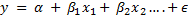
A regression model expresses a ‘dependent’ variable as a function of one or more ‘independent’ variables, generally in the form:
What we also see above in the Novartis example is the fitted regression line, ie the line that expresses the relationship between the y variable, called the dependent variable, in this case the returns for the Novartis stock; with the x variable, in this case the S&P 500 returns that are considered ‘independent’ or the regressor variable. What we are going to do next is go deeper into how regression calculations work. (For this article, I am going to limit myself to one independent variable, but the concepts discussed apply equally to regressing on multiple independent variables.)
Regression with a single dependent variable y whose value is dependent upon the independent variable x is expressed as
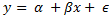
where α is a constant, so is β. x is the independent variable and ϵ is the error term (more on the error term later). Given a set of data points, it is fairly easy to calculate alpha and beta – and while it can be done manually, it can be done using Excel using the SLOPE (for calculating β)and the INTERCEPT (α) functions.
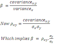
If done manually, beta is calculated as:
β = covariance of the two variables / variance of the independent variable
Once beta is known, alpha can be calculated as
α = mean of the dependent variable (ie y) – β * mean of the independent variable (ie x)
Beta and correlation
At this point it is important to point out the relationship between beta and correlation.
Predicted versus the observed value
Now let us go back to the initial equation:
Now that we have seen how to calculate α and β (ie, either using the formulae, or using Excel), it is probably possible to say that we can ‘predict’ y if we know the value of x. The ‘predicted’ value of y is provided to us by the regression equation. This is unlikely to be exactly equal to the actual observed value of y. The difference between the two is explained by the error term – ϵ. This is a random ‘error’ – error not in the sense of being a mistake – but in the sense that the value predicted by the regression equation is not equal to the actual observed value. This error is ‘random’ and not biased, which means that if you sum up ϵ across all data points, you get a total of zero. Some observations are farther away from the predicted value than others, but the sum of all the differences will add up to zero. (If it weren’t zero, the model would be biased in the sense it was likely to either overstate or understate the value of y.)
Intuitively, the smaller the individual observed values of ϵ, even though adding up to zero, the better is our regression model. How do we measure how small the values of ϵ are? One obvious way would be to add them up and divide by the number of observations to get an ‘average’ value per data point – but that would just be zero as just explained. So what we do is the next best thing: take a sum of the squares of ϵ and divide by the number of observations. For a variable whose mean is zero, this is nothing but its variance.
This number is called the standard error of the regression – and you may find it referred to as ‘standard error of the regression line’, ‘standard error of the estimate’ or even ‘standard error of the line’, the last phrase being from the PRMIA handbook.
This error variable ϵ is considered normally distributed with a mean of zero, and a variance equal to σ2.
The standard error can be used to calculate confidence intervals around an estimate provided by our regression model, because using this we can calculate the number of standard deviations either side of the predicted value and use the normal distribution to compute a confidence interval. We may need to use a t-distribution if our sample size is small.
Interpreting the standard error of the regression
The standard error of the regression is a measure of how good our regression model is – or its ‘goodness of fit’. The problem though is that the standard error is in units of the dependent variable, and on its own is difficult to interpret as being big or small. The fact that it is expressed in the squares of the units makes it a bit more difficult to comprehend.
(RMS error: We can also then take a square root of this variance to get to the standard deviation equivalent, called the RMS error. RMS stands for Root Mean Square – which is exactly what we did, we squared the errors, took their mean, and then the square root of the resultant. This takes care of the problem that the standard error is expressed in square units.)
Coming back to the standard error – what do we compare the standard error to in order to determine how good our regression is? How big is big? This takes us to the next step – understanding the sums of squares – TSS, RSS and ESS.
TSS, RSS and ESS (Total Sum of Squares, Residual Sum of Squares and Explained Sum of Squares)
Consider the diagram below. Yi is the actual observed value of the dependent variable, y-hat is the value of the dependent variable according to the regression line, as predicted by our regression model. What we want to get is a feel for is the variability of actual y around the regression line, ie, the volatility of ϵ. This is given by the distance yi minus y-hat. Represented in the figure below as RSS. The figure below also shows TSS and ESS – spend a few minutes looking at what TSS, RSS and ESS represent.
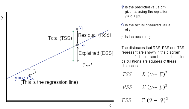
Now ϵ = observed – expected value of y
Thus, ϵ = yi – y^ . The sum of ϵ is expected to be zero. So we look at the sum of squares:
The value of interest to us is = Σ (yi – y^ )2. Since this value will change as the number of observations change, we divide by ‘n’ to get a ‘per observation’ number. (Since this is a square, we take the root to get a more intuitive number, ie the RMS error explained a little while earlier. Effectively, RMS gives us the standard deviation of the variation of the actual values of y when compared to the observed values.)
If s is the standard error of the regression, then
s = sqrt(RSS/(n – 2))
(where n is the number of observations, and we subtract 2 from this to take away 2 degrees of freedom*.)
Now
How good is the regression?
Intuitively, the regression line given by α + βx will be a more accurate prediction of y if the correlation between x and y is high. We don’t any math to say that if the correlation between the variables is low, then the quality of the regression model will be lower because the regression model is merely trying to fit a straight line on the scatter plot in the best possible way.
Generally, R2, called the coefficient of determination, is used to evaluate how good the ‘fit’ of the regression model is. R2 is calculated as ESS/TSS, ie the ratio of the explained variation to the total variation.
R2 = ESS/TSS
R2 is also the same thing as the square of the correlation (stated without proof, but you can verify it in Excel). Which means that our initial intuition that the quality of our regression model depends upon the correlation of the variables was correct. (Note that in the ratio ESS/TSS, both the numerator and denominator are squares of some sort – which means this ratio explains how much of the ‘variance’ is explained, not standard deviation. Variance is always in terms of the square of the units, which makes it slightly difficult to interpret intuitively, which is why we have standard deviation.)
How good are the coefficients?
Our regression model provides us values for α and β. These, after all, are only estimates. We can assess how good these estimates are, and how ‘significant’ they are. As estimates, the calculated values represent point estimates that have a range of possibilities for the true value to be on either side of this estimate – depending upon their standard deviation.
We can calculate the standard deviation of both alpha and beta – but the formulae are pretty complex if calculated manually. Excel does a great job of providing these standard deviations as part of its Data Anaslysis, Regression functionality as we shall see in a moment.
Once the standard deviations, or the standard errors of the coefficients are known, we can determine confidence levels to determine the ranges within which these estimated values of the coefficients lie at a certain level of significance.
Intuitively, we know that alpha and beta are meaningless if their value is zero, ie, if beta is zero, it means the independent variable does not impact the dependent variable at all. Therefore one test often performed is determining the likelihood that the value of these coefficients is zero.
This can be done fairly easily – consider this completely made up example. Assume that the value of beta is 0.5, and the standard error of this coefficient is 0.3. We want to know if at 95% confidence level this value is different from zero. Think of it this way: if the real value were to be zero, how likely is it that we ended up estimating it to be 0.5? Well, if the real value were to be zero, and were to be distributed according to a normal distribution, then 95% of the time we would have estimated it to be in the range within which the normal distribution covers 95% of the area under the curve on either side of zero. This area extends from -1.96 standard deviations to +1.96 standard deviations on either side of zero. This should be -0.59 (=0.3*1.96) to +0.59. Since the value we discovered was 0.5, it was within the range -0.59 to 0.59, which means it is likely that the real value was indeed zero, and that our calculation of that as 0.5 might have been just a statistical fluke. (What we did just now was hypothesis testing in plain English.)
Determining the goodness of the regression – The ‘significance’ of R2 & the F statistic
Now the question arises as to how ‘significant’ is any given value of R2? When we speak of ‘significance’ in statistics, what we mean is the probability of the variable in question being right. It means that we believe that the variable or parameter in question has a distribution, and we want to determine if the given value falls within the confidence interval (95%, 99% etc) that we are comfortable with.
Estimates follow distributions, and often we see statements such as a particular variable follows the normal or lognormal distribution. The value of R2 follows what is called an F-distribution. (The answer to why R2 would follow an F distribution is beyond the mathematical abilities of this author – so just take it as a given.) The F-distribution has two parameters – the degrees of freedom for each of the two variables ESS and TSS that have gone into calculating R2. The F-distribution has a minimum of zero, and approaches zero to the right of the distribution. In order to test the significance of R2, one needs to calculate the F statistic as follows:
F statistic = ESS / (RSS/(T-2)), where T is the number of observations. We subtract 2 to account for the loss of two degrees of freedome. This F statistic can then be compared to the value of the F statistic at the desired level of confidence to determine its significance.
All of the above about the F statistic is best explained with an example:
Imagine ESS = 70, TSS = 100, and T=10 (all made up numbers).
In this case, R2 = 0.7 (=70/100)
Since ESS + RSS = TSS, RSS = 30 (= 100 – 20)
Therefore the F statistic = 20/(30/(10-2)) = 5.33
Assume we want to know if this F statistic is significant at 95%, in other words, could its value have been zero and we accidentally happened to pick a sample that we got an estimate that was 5.33? We find out what the F statistic should be at 95% – and compare that to the value of ‘5.33’ we just calculated. If ‘5.33’ is greater than the value at 95%, we conclude that R2 is significant at the 95% level of confidence (or is significant at 5%). If ‘5.33’ is less than what the F value is at the 95% level of confidence, we conclude the opposite.
The value of F distribution at the desired level of confidence (= 1 – level of significance) can be calculated using the Excel function =FINV(x, 1, T – 2). In this case, =FINV(0.05,1,8)= 5.318. Since 5.33>5.318, we conclude that our R2 is significant at 5%.
We then go one step further – we can determine at what level does this F statistic become ‘critical’ – and we can do this using the FDIST function in Excel. In this case, =FDIST(5.33,1,8) =0.0498, which happens to be quite close to 5%. The larger the value of the F statistic, the lower the value the FDIST function returns, which means a higher value of the F statistic is more desirable.
Summing up the above:
- We figured out how to get estimates of alpha and beta, and therefore be able to calculate the regression equation,
- We calculated the Residual Sum of Squares, that provides us with an idea of how scattered around our regression line the real observations are,
- We calculated the root of RSS to get RMS error that provides us an idea of the ‘average’ error observed in each estimate – the larger this is, the poorer our regression model,
- We calculated R2, the square of correlation, which tells us how good our regression model is by informing us of the ratio between explained variance and total variance in the dependent variable (note: R2 talks about variance, not standard deviation).
- We also saw how correlation and beta are connected together.
- We then figured out how to calculate confidence limits relating to our estimates of alpha and beta.
- We also saw how to estimate the significance of R2.
Putting it all together: interpreting Excel’s regression analysis output
Consider a made up example of two variables x and y as follows, on which we perform a regression analysis in Excel (go to Data Analysis, and select Regression. You will need to make sure that the add-in for data analysis is installed for Excel to use. If you don’t know how to do that, Google for how to install the ‘Data Analysis’ Add-in in Excel.
)
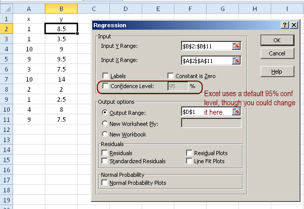
We then perform the regression analysis and get the results as follows. I have provided explanations of all the parameters that the Excel provides as an output, either in the picture below or as notes referenced therein.
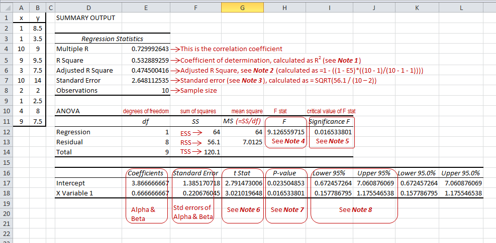
Note 1: Coefficient of determination (cell E5)
The coefficient of determination is nothing but R^2, something we discussed in detail earlier (ie, the ESS/TSS), and equal to the square of the correlation.
Note 2: Adjusted R2 (cell E6)
Adjusted R2 is a more refined way of calculating the coefficient of determination. It is possible to increase R2 by including more explanatory variables in the regression, and while the value of R2 may increase due to this, it may not make the model any superior because all we have achieved is a misleading overfitted model that may not provide any better predictions.
The adjusted R2 takes into account the number of independent variables in the model, and the sample size, and provides a more accurate assessment of the reliability of the model.
Adjusted R^2 is calculated as 1 – (1 – R^2)*((n-1)/(n-p-1)); where n is the sample size and p the number of regressors in the model.
Ie, Adjusted R2 = ![]()
In this case, Adj R2 =1 – ((1 – E5)*((10 – 1)/(10 – 1 – 1))) = 0.4745
Note 3: Standard error (cell E7)
Standard error = SQRT(RSS/(T – 2)) where T is the sample size. We reduce 2 from the sample size to account for the loss of two degrees of freedom, one for the regression estimate itself, and the second for the explanatory variable.
In this case, standard error = SQRT(56.1 / (10 – 2)) = 2.648
Note 4: F (cell H12)
The F statistic is explained earlier in this article. Calculated as ESS / (RSS/(T-2)), in this case that is =64/(56.1/8) (where 8 was obtained as T-2=10-2=8)
Note 5: Significance F
Significance F gives us the probability at which the F statistic becomes ‘critical’, ie below which the regression is no longer ‘significant’. This is calculated (as explained in the text above) as =FDIST(F-statistic, 1, T-2), where T is the sample size. In this case, =FDIST(9.126559714795,1,8) = 0.0165338014602297
Note 6: t Stat
The t Stat describes how many standard deviations away the calculated value of the coefficient is from zero. Therefore it is nothing but the coefficient/std error. In this case, these work out to 3.86667/1.38517=2.7914 and 0.6667/0.22067 = 3.02101 respectively.
Why is this important? This is because if the coefficient for a variable is zero, then the variable doesn’t really affect the predicted value. Though our regression may have returned a non-zero value for a variable, the difference of that value from zero may not be ‘significant’. The t Stat helps us judge how far is the estimated value of the coefficient from zero – measured in terms of standard deviations. Since the value of the coefficients follows the t distribution, we can check, at a given level of confidence (eg 95%, 99%), whether the estimated value of the coefficient is significant. All of Excel’s regression calculations are made at the 95% level of confidence by default, though this can be changed using the initial dialog box when the regression is performed.
Note 7: p value
In the example above, the t stat is 2.79 for the intercept. If the value of the intercept were to be depicted on a t distribution, how much of the area would lie beyond 2.79 standard deviations? We can get this number using the formula =TDIST(2.79,8,2) = 0.0235. That gives us the p value for the intercept.
Note 8: Lower and upper 95%
Assume the coefficient (either the intercept or the slope) has a mean of 0, and a standard deviation as given. Between what values either side of 0 will 95% of the area under the curve lie? This question is answered by these values.
If the estimated value of the coefficient lies within this area, then there is a 95% likelihood that the real value could be anything within this area, including zero. These ranges allow us to judge whether the values of the coefficients are different from zero at the given level of confidence.
How is this calculated? In the given example, we first calculate the number of standard deviations for the given confidence level either side of zero that we can go, and we assume a t distribution. In this case, there are 8 degrees of freedom and therefore the number of SDs is TINV(0.05,8) = 2.306. We multiply this by the standard error for the coefficient in question and add and subtract the result from the estimate. For example, for the intercept, we get the upper and lower 95% as follows:
Upper 95% = 3.866667 + (TINV(0.05,8) * 1.38517) = 7.0608 (where 3.866667 is the estimated value of the coefficient per our model, and 1.38517 is its standard deviation)
In the same way,
Lower 95% = 3.866667 – (TINV(0.05,8) * 1.38517) = 0.67245
We do the same thing for the other coefficient, and get the upper and lower 95% limits
Lower 95% = 0.66667 – (TINV(0.05,8) * 0.220676) = 0.15779
Upper 95% = 0.66667 + (TINV(0.05,8) * 0.220676) = 1.174459
*A note about degrees of freedom: A topic that has always confused me, but has never been material enough to warrant further investigation. This is because as you subtract 1 or 2 from your sample size n, its impact vanishes rapidly as n goes up. For most practical situations it doesn’t affect things much, so I am happy to accept it as explained in textbooks.