The topic of kurtosis can cause some confusion. Think fat and thin tails, and “peakedness” and leptokurtosis. How is it that having a ‘pointier’ peak means having fat tails, and how is that different from a normal distribution that just has a smaller standard deviation? And how does a t-distribution manage to have fatter tails when its peak can in fact be lower than that of the normal distribution?
All of this has to do with the shape of the distribution under consideration. A key determinant of the shape of a distribution is its variance, but there is more to shape than just variance. Two distributions with identical means and variances can have very different shapes, and kurtosis is one of the measures of that difference. It looks at how much of the ‘weight’ of the distribution (recall that the total weight, or the area under the curve, is 1) is sitting in the tails as opposed to the middle of the distribution.
The formula for kurtosis is given below, but the emphasis of this article is to focus on an intuitive understanding of kurtosis, and peakedness and tails, so let me state the formula and get it out of the way. Kurtosis is defined as the fourth moment around the mean, or equal to:

The kurtosis calculated as above for a normal distribution calculates to 3. Because kurtosis compares a distribution to the normal distribution, 3 is often subtracted from the calculation above to get a number which is 0 for a normal distribution, +ve for leptokurtic distributions, and –ve for mesokurtic ones.
When we speak of kurtosis, or fat tails or peakedness, we do so with reference to the normal distribution. We compare other distributions to the normal distribution, so it is important to be clear about the shape of the normal distribution. So let us spend a few minutes talking about the shape of the normal distribution.
The shape of the normal distribution:
The normal distribution, as you are probably tired of hearing, has a familiar bell-shaped distribution. But what you may not have noticed is that this bell shape is identical for all normal distributions with the same variance. If the variance is not the same, the shape is still the same provided you scale the axes correctly.
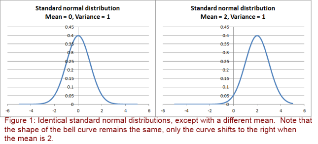
For example, look at the following normal distributions – both with the same variance but different means. They are identical, though situated at different places on the x-axis due to the difference in means. But the shapes are identical.
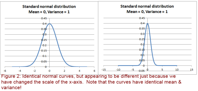
In the same way, identical distributions may be made to look different, as is illustrated in the figure below.
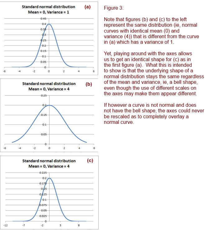
Now consider two normal distributions with different variances. It seems that the one with the larger variance is a bit more spread out (as expected), and may look to be of a different shape. But actually, the real shape is identical – because if you squeeze the scale on the x-axis, you get the same identical shape, which is the bell shape of the normal distribution.
Here is another diagram that brings out the difference between variance and kurtosis:
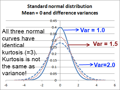
What I would like to emphasize is that variance is not kurtosis. Variance does indeed spread a distribution out, but kurtosis measures something different, and does this measurement with reference to a normal curve with identical variance. Here is another diagram that puts normal curves with different variances side by side. All of these have the same kurtosis (of 3, or 0, whichever way you prefer to measure it).
Enter kurtosis
Having discussed the shape of a normal distribution, we can talk about kurtosis and what it means to have fat tails and peakedness. The total area under a curve is by definition equal to one.
With that in mind, think about what having fatter tails might mean. If you were to think of a curve having three parts (all imaginary) – the peak, the shoulder (or the middle part), and the tails, you can imagine what happens if you stretch the peak up. That reduces variance, and probably sucks in ‘mass’ from the shoulders. But in order to keep the variance the same, the tails rise higher, increasing variance and also providing fatter tails.
Fat tails would imply there is more area under the tails, which means something else has to reduce elsewhere – which means that the ‘shoulders’ shrink making the peak taller. In order to compare kurtosis between two curves, both must have the same variance. At the risk of being repetitive, note that the variance has an impact on the shape of a curve, in that the greater the variance the more spread out the curve is. When we say that kurtosis is relevant only when comparing to another curve with identical variance, it means that kurtosis measures something other than variance.
Therefore peakedness is associated with fatter tails (and not thinner ones), which is why leptokurtic distributions have a higher kurtosis.
Distributions can come in all sorts of shapes, and they may or may not be symmetrical. In many cases, kurtosis cannot be estimated just by looking at the shape of the distribution and will need to be calculated. While often peaking distributions will have fatter tails, the t-distribution is flatter and yet has fatter tails as shown below.
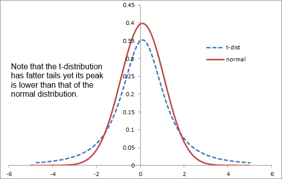
Note how the mass, or weight has moved around to the tails above. Generally, for distributions that have a higher peak the middle part of the distribution is squeezed and is closer to the mean, which would have the effect of bringing the variance down, and that gets offset by more observations in the tails, hence the fatter tails.
Hope the above is useful to all!