This brief article intends to clarify the differences between some concepts relating to credit VaR. One thing to note about credit risk is that you need to watch out whether you are inferring VaR from a distribution of the value of the portfolio, or from a distribution of the losses in the portfolio. One is a mirror image of the other, they give the same results, but they are not identical and you should intuitively understand the difference.
Consider a hypothetical portfolio of $100m in a retail credit portfolio, which is made up of a large number of small loans. For each loan, there is a probability of expected loss, however, an important thing to note is that for each individual loan the eventual loss will be either 0% or 100%. Over the portfolio of these loans however, the average losses will be realized as some individual loans would have failed completely, and others would pay off in their entirety.
Portfolio value and portfolio losses: If the portfolio has a value of $100m to start with, then over a certain future horizon this value will change as losses are realized. The maximum future value will however be only $100m, which will correspond to losses of $0m. By the same token, the minimum value of the portfolio will be $0, corresponding to losses of $100m. In all likelihood, the actual realized losses will be between these two extremes.
Again, losses will happen, with the expected value equal to the $100m minus whatever the expected losses on this portfolio are. Assume for a moment that we know (whether from data, estimates, or historical experience) that 15% of these loans will go bad and we will be able to recover nothing. The other 85% of the loans will be paid off in full. In such a case, the ‘expected value’ of the portfolio will be $85m. Now this loss of $15m is not known with certainty, and the 15% estimate will have a variance that will cause the final actual value to be different. Over time, or over many years, however the expected losses will be 15%. What we are interested in is a distribution of what the future value of the portfolio will be at the end of our time horizon so we can figure out the worst case losses or portfolio value with a certain level of confidence.
At this point, see the correspondence between portfolio value and portfolio losses – the total of losses and the future value will always be the $100m, in other words, if the future value of the portfolio is say $x, then the losses have been $100m – $x.
Since value-at-risk is the worst case losses at a certain confidence level over a given time horizon, we can calculate value-at-risk if we have a distribution of future portfolio value, or a distribution of future portfolio losses – because after all these two distributions can be derived from each other and represent the same set of outcomes but presented differently.
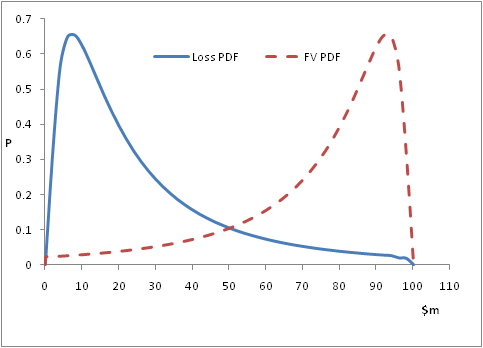
Consider the curves below – I have used the lognormal distribution to represent the loss distribution on the portfolio only as an illustration, but it does not have to be that, it can be anything else too. The loss distribution shows that there is a certain level of expected loss that will be realized with a high probability, and as we go further away from the expected loss, the probability keeps going down. The same data can also be represented as a distribution of the future value of the credit portfolio, and one can quite easily deduce the value-at-risk from that distribution as well.
With the above conceptual understanding, let us look at some terms that are used in credit risk. I would strongly recommend that you follow the example, ie work the numbers in the illustration I have provided so you can distinguish between the different terms.
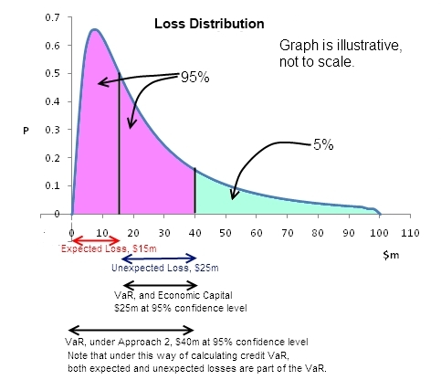
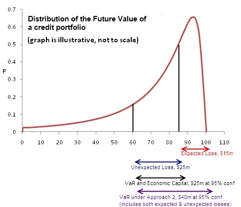
Expected losses are the losses expected on a credit portfolio, say if we believe 15% of the portfolio will go bad, then expected losses are going to be $15m. These should be provided for in the P&L, and considered in the pricing of the loans. These losses are ‘expected’, ie we know that these will happen, and even if they don’t fully materialize in one year, they should be fully provided for as they would show up in future periods.
Unexpected losses: Intuitively, one might say that unexpected losses are any losses that occur in excess of this $15m. But that is not correct. Unexpected losses are calculated at a given confidence interval, and are equal to the losses at the given confidence interval minus expected losses. Therefore if the value of the portfolio at 95% confidence level is $60, then total losses are $40m, and unexpected losses are $25m. (Unexpected losses are not VaR minus expected losses.)
Credit VaR can be calculated according to two approaches as follows:
Approach 1 (preferred and should be your default): Credit VaR is the distance from the mean to the percentile of the forward distribution, at the desired confidence level (paraphrased from the PRMIA Handbook). This is nothing but the unexpected credit loss at the desired confidence level. The mean in this case is represented by $15m, and the 95th-percentile losses are $40m, therefore Credit VaR is also $25m. Your understanding of credit VaR should follow this approach as it is the most reasonable and consistent.
Approach 2: However, there is another way to look at credit VaR: it can also be understood to be the 95th percentile itself, ie including the expected losses. In this case, the 99th percentile losses are $40m, therefore credit VaR could also be considered to be $40m as these are the total losses at that level of confidence. Both approaches have been used in the PRMIA handbook, and you will find both approaches depending upon which textbook you consult.
For the exam, you should be aware of both ways of calculating credit VaR, and hopefully the answers will match the result from only one of these approaches. If both approaches show up, then my recommendation is to use Approach 1.
Economic capital is required in respect of the unexpected credit losses as a buffer to absorb unexpected losses, and is therefore also equal to the unexpected losses PROVIDED the time horizon is the same. For credit risk, the time horizon is normally 1 year (as opposed to 2 weeks, or 10 working days for market risk) and therefore economic capital is the same at $25m.
So how do all of the above fit in with our distributions? Here – look at the graphics below that explain the concept from both a future value perspective, and a loss distribution point of view.
If the above is not clear, write to me and I will explain further.