A lot of finance and risk management is about distributions. For the PRMIA exam, you really need to understand the concepts underlying distributions, what different shapes mean, what the parameters are, what a cdf is (vs a pdf) and which to use when. Of course, the most commonly used distribution assumption is that returns are normally distributed, so this article talks about the normal distribution and also other important distributions. More importantly, I have provided spreadsheets that model each of the distributions so you can play around and see the behaviour of the distribution as you change the parameters underlying it.
Financial variables such as returns are often modeled using one or the other distribution. A distribution is a graph of the probability of the return being a particular value, or being in a range of values.
This tutorial discusses some common distributions that are encountered in finance. Distributions have different shapes, which means that the probabilities of the variable they describe are differently distributed. By different ‘shapes’, we mean things such as whether the distribution looks skewed or is symmetrical, whether it has sharp peaks or flat peaks, one peak or multiple peaks, discontinuities etc. There is no limitation to the different shapes that a distribution may take, but the practical problem many ‘complex’ looking distributions create is that they may not have an easy equation that defines them. Having an equation for a distribution means the distribution is ‘closed form’, which makes it easy to deal with to calculate probabilities, confidence intervals, & manipulate using software for tasks such as doing monte carlo simulations.
Remember that for most variables we do not know what the actual distribution looks like. In some cases, we will never know as only one path of events occurring will reveal itself in the future, while the distribution is an ex-ante anticipation of the probabilities of different things happening in the future. Therefore the distribution is almost always an assumption. For example, we often assume that returns are normally distributed. They may not be. We may drop the normality assumption to use, say, a t-distribution because we like slightly fatter tails. But even here, we are assuming, we do not know what the future will bring. Yet assuming a distribution with reason can make the problem of assessing and measuring risk tractable and manageable.
The distributions that are generally referred to in finance are all closed form, ie there is a neat equation that describes them. These equations have parameters. The parameters influence the shape of the distribution. When we think about a distribution, we should think about its shape and its parameters, and if they are easy to estimate.
Distributions are broadly of two types:
- Discrete: Here, a variable may only have discrete values, for example the number of heads in 10 tosses of a coin. The number of realized heads in ten tosses of a coin will never be 7.73. It will always be a whole number, which can vary between 0 and 10, but can never reach a value like 7.73 heads.
- Continuous: Continuous variables are those that can have any value, for example the share price of a company. That price can well be $7.73, just as it can be 0 or 10. One might argue that it cannot be $7.735, because half a cent cannot be received or paid. To that extent, even this variable can be considered discrete, but we generally do not do so. We consider variables such as prices, interest rates, returns, FX rates to be continuous even though market convention and monetary considerations may slightly limit the values these variables can take.
What does the distinction between discrete and continuous variable really imply? The one thing it means is that for a discrete variable we can create a histogram with a bar for each value that the variable may take. For a continuous variable, we cannot create a histogram but draw a curve. Often, if the bars of the histogram are close together, we can approximate a curve by “joining the tops” of the bars, and also vice-versa. In fact, a continuous function is nothing but a limiting case of a discrete function where the number of discrete values approach infinity.
In finance and risk management, continuous distributions are often used to model discrete variables, and vice versa too.
When talking of distributions, it is important to know the following terms:
- Relative frequency: Relative frequency is just the total frequency for a value of the variable divided by the total number of observations. As a result, relative frequencies add to 1, which is what the case is for probabilities as well. For our purposes and for the PRMIA exam, consider relative frequency to be a proxy for probability.
- Probability mass function: This applies to discrete variables, and is a function (or a graph thereof) that gives the probabilities of the variable acquiring certain values.
- Probability density function (pdf): This is the same thing as the probability mass function, but only for continuous variables. Since most of our work relates to continuous variables, a pdf is what we will run into the most. A pdf is interpreted as providing the probability of the variable being between two values by measuring the area under the curve. The total area under the curve is by definition 1.
- Cumulative distribution function (cdf): This is the cumulative probability of a continuous variable being equal to or less than the value being considered. For a cdf, we do not talk in terms of ‘area under the curve’, because that can be read directly off the cdf. The cdf starts at zero on the left, and approaches 1 towards the right.
Below we discuss the key distributions we encounter in finance, the parameters that define them, and an Excel model of what the distribution looks like. Play around with the Excel model, change the parameters and see how the distribution changes shape as you do so.
The Binomial Distribution
The binomial distribution models an event whose outcome is either a success or a failure. For example, consider the toss of a coin which has two mutually exclusive outcomes, and where the probability of the outcomes for any trial is not affected by prior trials. There are n+1 outcomes for n trials, and 2^n different paths to get to the final outcomes. The binomial distribution is used extensively for valuing path dependent options using ‘binomial trees’.
Parameters:
‘p’ is the probability of success in each trial
‘r’ is the number of successes
‘n’ is the number of trials

Expectation = np
Variance = np(1-p)

The binomial distribution can be modeled in Excel using the function ‘BINOMDIST’.
Here is a spreadsheet if you wish to play around with an Excel model.

Poisson distribution
The Poisson distribution (pronounced poo-aa-sson, not poison) is another discrete distribution that is used to model the probability of n number of events that can happen in a particular time interval, provided we know what the average is. For example, if we know that the average number of accidents that happen on a stretch of road is 5 per day, then Poisson distribution can answer questions such as ‘what is the probability of having 6 accidents in an hour’.
Poisson distributions have just one parameter – λ – which is the mean and also the variance of the distribution. The probability of ‘k’ successes is given by the formula

Poisson distribution can be used to model certain operational risks. The Poisson distribution can be modeled in Excel using the function ‘POISSON’. A significant advantage that the Poisson distribution offers is the fact there there is only one parameter that defines the distribution. This parameter λ is also the mean and variance of the distribution.
Here is a spreadsheet if you wish to play around with an Excel model.

The Uniform distribution
The uniform distribution is one where every possibility between two values can occur with equal likelihood. For example, the probability of throwing any value between 1 and 6 on the throw of a die is a uniform distribution, where 1 and 6 are the bounds of the values the variable can take. In this case, the variable is discrete. A uniform distribution is used extensively in simulation in finance, often even without knowing it, for example when a random number is to be drawn such that each random number has the same probability of being selected.
If m and n be the two bounds of the uniform distribution, then


The normal distribution
The familiar normal distribution has just two parameters: the mean and standard deviation. A ‘standard’ normal distribution is a normal distribution with a mean of zero and standard deviation of exactly 1.
The pdf for the normal distribution is given by the rather daunting function given below, though in practice there are a number of Excel functions available (ie NORMDIST & NORMINV) that the risk manager can use.

Where the different variables used have their usual meaning.
The normal distribution is often used to model asset returns that are mean reverting and have a constant volatility.
Here is a spreadsheet if you wish to play around with an Excel model.

The lognormal distribution
The lognormal distribution is used to model asset prices whose returns are normally distributed. The lognormal distribution can be modeled in Excel using the function ‘LOGNORMDIST’. Average asset returns become the ‘drift’ for modeling prices, with a given volatility. Like the normal distribution, the lognormal distribution has two parameters – the mean and variance (or standard deviation).
The PDF function for the lognormal distribution is a rather daunting expression that you need not remember for the PRM exam.
Here is a spreadsheet if you wish to play around with an Excel model.

The Beta distribution
The beta distribution has two parameters, α and β, and depending upon the values assigned to these two variables, the distribution can take many different shapes. This distribution can be used to simulate random recovery rates when assessing credit risks.

The values of α and β can be calculated directly from the values of the mean and standard deviation.


Here is a spreadsheet if you wish to play around with an Excel model.

Student’s t-distribution
The t-distribution is used generally where sample sizes are less than 30 and the population is considered normal. However, unlike the normal distribution the t-distribution has fatter tails, something that gives higher values of value-at-risk at high confidence levels. Therefore some risk managers use the t-distribution to model asset returns to take care of heavy tails.
The t-distribution has a daunting expression for its probability distribution function, which is unlikely to be asked in the PRMIA exam. It can be modeled in Excel using the function ‘TDIST’. The t-distribution has only one parameter – called degrees of freedom, which is equal to the sample size minus 1.
Here is a spreadsheet if you wish to play around with an Excel model.

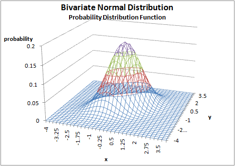
The bivariate normal distribution
A bivariate distribution is one where the function is dependent upon two variables, and not just one as we have seen so far. For example, y = a + bx is a univariate function, while y = a + bx +cz is a bivariate function with two variables x and z. Graphing a bivariate distribution takes a three-dimensional graph, with one axis each for each of the variables, and the vertical ‘z’ axis for the probability. A normal bivariate has the characteristic bell shape of the normal distribution, only in three dimensions so it looks like a sloping mountain.
Here is a spreadsheet in case you wish to play around.
The bivariate normal distribution is used for credit risk estimations as part of the CreditMetric methodology.